By Jakob Schwichtenberg, author of No-Nonsense Classical Mechanics (393 pages) and No-Nonsense Quantum Field Theory (642 pages). Page references match the current editions.
The Euler–Lagrange equation is the workhorse of theoretical physics:
$$\frac{\partial L}{\partial q} - \frac{d}{dt}\!\left(\frac{\partial L}{\partial \dot{q}}\right) = 0 \qquad \Longleftrightarrow \qquad \frac{d}{dt}\!\left(\frac{\partial L}{\partial \dot{q}}\right) = \frac{\partial L}{\partial q}.$$Whenever nature minimizes or extremizes an integral—whether it is the shortest path on a curved surface (geodesics in general relativity), the path of stationary action in Lagrangian mechanics, Maxwell's equations from the electromagnetic Lagrangian, or the Klein–Gordon and Dirac equations in quantum field theory—the Euler–Lagrange equation is how you turn "the integral is stationary" into an ordinary or partial differential equation you can actually solve.
Many textbooks obscure this derivation behind mysterious $\delta$-operators ($\delta\dot{q} = \frac{d}{dt}\delta q$) before defining what $\delta$ means. Below (following Section 4.3, p81–p88 of No-Nonsense Classical Mechanics), we turn the entire variational problem into ordinary single-variable calculus with a small real parameter $\epsilon$, so not a single step requires faith.
1. Turning functional calculus into ordinary $\frac{d}{d\epsilon}$ calculus
Suppose a system starts at a known configuration $q_1$ at time $t_1$ and arrives at $q_2$ at time $t_2$. Out of all smooth paths connecting $(t_1, q_1)$ to $(t_2, q_2)$, let $q(t)$ be the true physical path that makes the action
$$S[q] = \int_{t_1}^{t_2} L\!\big(q(t), \dot{q}(t), t\big)\,dt$$stationary. To compare $q(t)$ against every nearby path with the same endpoints, pick an arbitrary smooth deformation function $\eta(t)$ satisfying
$$\eta(t_1) = 0 \qquad \text{and} \qquad \eta(t_2) = 0,$$and build a one-parameter family of deformed paths:
$$q_\epsilon(t) \equiv q(t) + \epsilon\,\eta(t), \qquad \dot{q}_\epsilon(t) = \dot{q}(t) + \epsilon\,\dot{\eta}(t).$$For $\epsilon = 0$, we recover our true path $q_0(t) = q(t)$. Once $q(t)$ and $\eta(t)$ are fixed, the action along $q_\epsilon$ is just an ordinary real-valued function $S(\epsilon)$ of the single real variable $\epsilon$! Saying that $q(t)$ makes the action stationary against all endpoint-preserving variations simply means:
$$\left.\frac{dS(\epsilon)}{d\epsilon}\right|_{\epsilon = 0} = 0 \qquad \text{for every smooth }\eta(t)\text{ with }\eta(t_1)=\eta(t_2)=0.$$2. The complete line-by-line annotated derivation
Now we differentiate $S(\epsilon)$ at $\epsilon = 0$. Follow each row from top to bottom; the right column states the exact calculus rule used on that line:
Why couldn't we stop at row 3 without integrating by parts? Because $\eta(t)$ and $\dot{\eta}(t)$ are not independent functions—once you draw a bump $\eta(t)$, its slope $\dot{\eta}(t)$ is already fixed! Integration by parts shifts $\frac{d}{dt}$ off $\eta(t)$ and onto $\frac{\partial L}{\partial\dot{q}}$, leaving a single arbitrary function $\eta(t)$ multiplying the entire bracket.
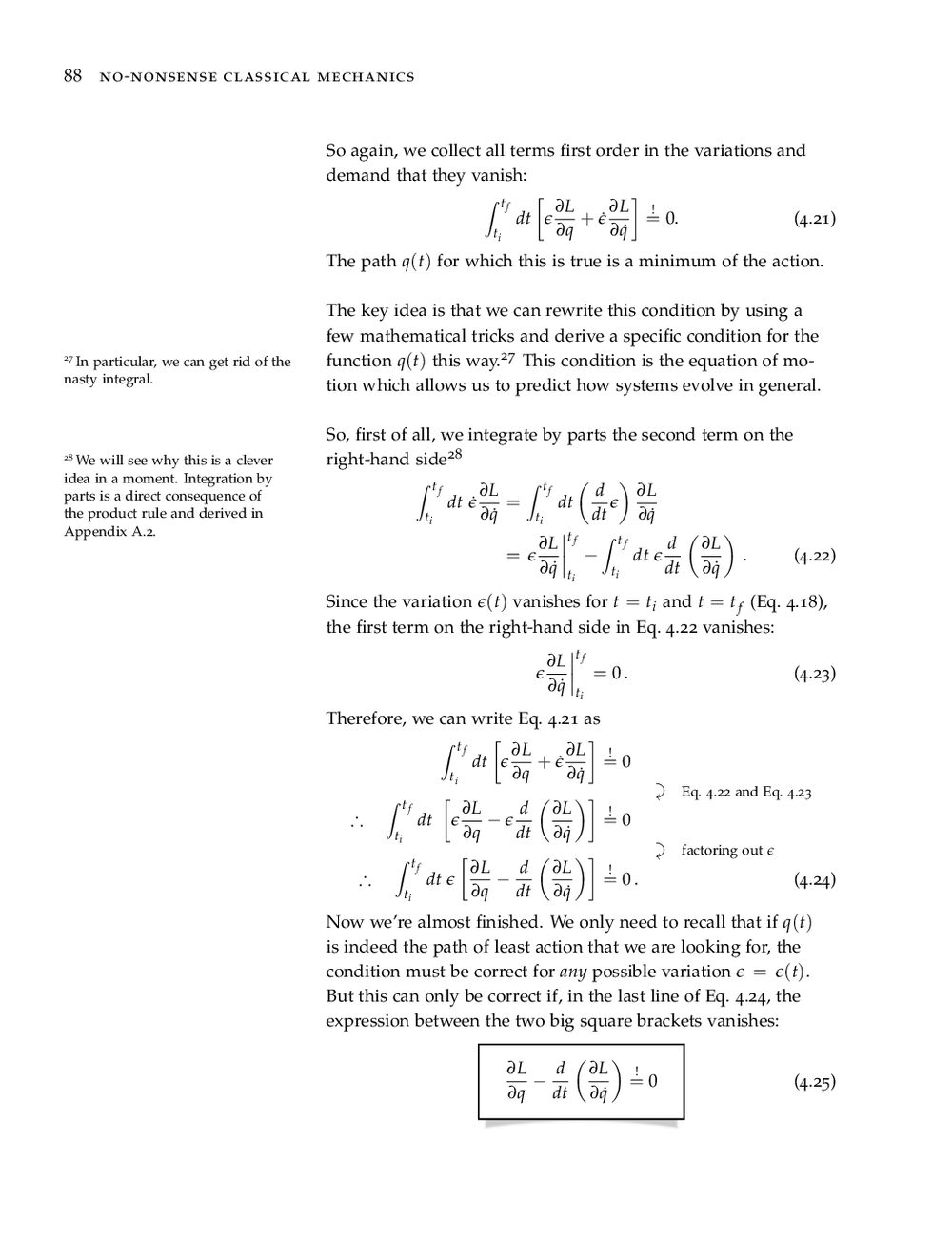
3. Many degrees of freedom ($N$ coordinates)
When a system has $N$ independent generalized coordinates $q = (q_1, \dots, q_N)$, we vary each coordinate $q_i(t) \to q_i(t) + \epsilon\,\eta_i(t)$ independently. Choosing $\eta_k(t)$ nonzero while setting $\eta_j(t) = 0$ for all $j \neq k$ isolates coordinate $k$, yielding $N$ coupled second-order differential equations:
$$\frac{\partial L}{\partial q_i} - \frac{d}{dt}\!\left(\frac{\partial L}{\partial \dot{q}_i}\right) = 0, \qquad i = 1, 2, \dots, N.$$Notice the biggest practical gift of this derivation: nowhere did we assume $q_i$ were Cartesian coordinates! Because $S[q]$ is a coordinate-independent integral, the Euler–Lagrange equation holds in identically the same form in polar $(r,\phi)$, spherical $(r,\theta,\phi)$, or center-of-mass coordinates.
4. Generalization to classical and quantum field theory
In electrodynamics and quantum field theory (Chapter 4, Section 4.3, p153 of No-Nonsense Quantum Field Theory), the dynamical variable is no longer $q(t)$ indexed by a discrete label $i$ at time $t$—it is a field $\phi(x^\mu)$ defined at every point $x^\mu = (ct, x, y, z)$ of spacetime. The action is the four-dimensional spacetime integral of a Lagrangian density $\mathcal{L}(\phi, \partial_\mu\phi)$:
$$S[\phi] = \int d^4x\;\mathcal{L}\big(\phi(x), \partial_\mu\phi(x)\big).$$Varying $\phi(x) \to \phi(x) + \epsilon\,\eta(x)$ (with $\eta(x) \to 0$ on the spacetime boundary) and integrating $\frac{\partial\mathcal{L}}{\partial(\partial_\mu\phi)}\,\partial_\mu\eta$ by parts via the four-dimensional divergence theorem produces the field-theory Euler–Lagrange equation:
$$\frac{\partial \mathcal{L}}{\partial \phi} - \partial_\mu\!\left(\frac{\partial \mathcal{L}}{\partial(\partial_\mu\phi)}\right) = 0.$$Quick check — the Klein–Gordon equation (p170 of QFT): Plug in the free real scalar Lagrangian density $\mathcal{L} = \frac{1}{2}(\partial_\mu\phi)(\partial^\mu\phi) - \frac{1}{2}m^2\phi^2$ (in natural units $\hbar = c = 1$ with metric $+---$). Then $\frac{\partial\mathcal{L}}{\partial\phi} = -m^2\phi$ and $\frac{\partial\mathcal{L}}{\partial(\partial_\mu\phi)} = \partial^\mu\phi$, so the Euler–Lagrange equation gives
$$-m^2\phi - \partial_\mu\partial^\mu\phi = 0 \quad\Longrightarrow\quad (\partial_\mu\partial^\mu + m^2)\phi = 0,$$the relativistic Klein–Gordon wave equation in two lines! Doing the exact same thing with $\mathcal{L}_{\text{EM}} = -\frac{1}{4}F_{\mu\nu}F^{\mu\nu} - J^\mu A_\mu$ yields the inhomogeneous Maxwell equations $\partial_\mu F^{\mu\nu} = \mu_0 J^\nu$.
Common questions
Why does the Euler–Lagrange equation say "stationary action" instead of "least action"?
Setting the first derivative $\left.\frac{dS}{d\epsilon}\right|_{\epsilon=0} = 0$ finds any stationary path—a local minimum, maximum, or saddle point, just like $f'(x_0)=0$ in ordinary calculus. For sufficiently short time intervals $t_2 - t_1$, the true path is genuinely a minimum of $S$, while over longer intervals (for example, past a focal/conjugate point of a harmonic oscillator after half a period) $S$ becomes a saddle point—yet $\delta S = 0$ and the Euler–Lagrange equation remain 100% exact!
What is the Beltrami identity?
When $L = L(q, \dot{q})$ has no explicit dependence on the independent variable $t$ ($\partial L/\partial t = 0$), Noether's theorem guarantees that the quantity $H = \dot{q}\frac{\partial L}{\partial\dot{q}} - L$ is conserved: $\frac{d}{dt}\!\left(\dot{q}\frac{\partial L}{\partial\dot{q}} - L\right) = 0$. That first integral is called the Beltrami identity, and it solves classic variational problems like the brachistochrone curve and catenary soap film without ever differentiating twice.
What is the difference between $\frac{\partial L}{\partial t}$ and $\frac{dL}{dt}$?
The partial derivative $\frac{\partial L}{\partial t}$ asks whether the formula for $L(q,\dot{q},t)$ contains the symbol $t$ explicitly when $q$ and $\dot{q}$ are held frozen (e.g., a time-varying external drive). The total derivative $\frac{dL}{dt} = \frac{\partial L}{\partial q}\dot{q} + \frac{\partial L}{\partial\dot{q}}\ddot{q} + \frac{\partial L}{\partial t}$ tracks how the numerical value of $L$ changes along a moving trajectory $q(t)$.
Go from calculus of variations to quantum fields
Want every fundamental derivation in mechanics and field theory worked out with zero skipped steps? Start with No-Nonsense Classical Mechanics (393 pages, 553 margin annotations) and continue with No-Nonsense Quantum Field Theory (642 pages, 1,089 margin annotations)—or get the entire four-book core curriculum in the $99 bundle.
CM Table of Contents (PDF) · Related guides: Lagrangian mechanics · Noether's theorem · Feynman diagrams.