By Jakob Schwichtenberg, author of No-Nonsense Quantum Field Theory (642 pages). Every step below carries a right-hand annotation in the style of the textbook; page numbers match the current paperback and eBook (natural units $\hbar = c = 1$).
Popular-science books present Feynman diagrams as little cartoons of electrons bouncing around in space and tossing "virtual photons" back and forth like basketballs. Then you open a graduate quantum field theory textbook, get hit with time-ordered exponentials, Wick contractions, and four-dimensional momentum integrals, and wonder how the cartoon has anything to do with the math.
Here is the honest truth (worked out first by brute force in Chapter 10, p407, and then turned into diagrams in Chapter 11, p421–p464 of No-Nonsense Quantum Field Theory):
What a Feynman diagram really is: A Feynman diagram is not a photograph of a physical process in space. It is a 1-to-1 visual shorthand for a specific algebraic term (or integral) in the perturbative Taylor-like series of a quantum scattering amplitude. The Feynman rules of a theory are simply the translation dictionary between picture pieces and algebraic factors.
1. Why physicists needed diagrams in the first place
In quantum field theory we want the scattering amplitude $\langle f | \hat{S} | i \rangle$—the probability amplitude that an initial state $|i\rangle$ of incoming particles with known momenta (say, two colliding particles $|p_1, p_2\rangle$) evolves into a final state $|f\rangle$ (say, $|p_3, p_4\rangle$). For free fields ($\mathcal{L}_0$), nothing scatters. As soon as you turn on an interaction Lagrangian density $\mathcal{L}_{\text{int}}$ (such as $-\frac{\lambda}{4!}\phi^4$ for a self-interacting scalar field, or $-e\bar{\psi}\gamma^\mu\psi A_\mu$ in quantum electrodynamics), exact solutions are almost never available.
When the coupling constant ($\lambda$ or $e$) is small, we switch to the interaction picture (Section 9.2, p382) and expand the time-evolution operator in powers of the interaction—the Dyson series (Section 9.3, p384):
$$\hat{S} = T\exp\!\left(i\int d^4x\;\mathcal{L}_{\text{int}}(\phi_I(x))\right) = \mathbf{1} + i\int d^4x\,\mathcal{L}_{\text{int}}(x) + \frac{i^2}{2!}\int d^4x\,d^4y\;T\!\big\{\mathcal{L}_{\text{int}}(x)\,\mathcal{L}_{\text{int}}(y)\big\} + \cdots$$If you try to evaluate $\langle p_3, p_4 | \hat{S} | p_1, p_2 \rangle$ directly by expanding every field operator $\phi_I(x)$ into creation and annihilation operators $a^\dagger_{\mathbf{k}}, a_{\mathbf{k}}$ and commuting them past one another by hand (as we deliberately do once in Chapter 10, p407, so you see there is zero magic!), a single first-order term takes five pages of index-heavy algebra—and second order explodes into dozens of terms.
Wick's theorem (Section 11.2, p428; proven in Appendix B, p611) tames that explosion: the vacuum expectation value of a time-ordered product of free fields equals the sum over all complete pairings ("contractions") of those fields. And each contraction between spacetime points $x$ and $y$ is a single known function—the Feynman propagator $D_F(x - y) \equiv \langle 0 | T\{\phi_I(x)\,\phi_I(y)\} | 0 \rangle$ (p334 & p430)!
Feynman's stroke of genius was to draw each spacetime interaction point $x$ as a dot (vertex), each external state $|p_i\rangle$ as an external leg, and each contraction $D_F(x-y)$ connecting two points as an internal line. Suddenly, counting all distinct pairings in Wick's theorem reduces to drawing all topologically distinct graphs!
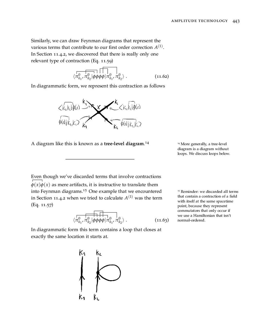
2. The translation dictionary: momentum-space Feynman rules
In practice we Fourier-transform from spacetime positions $x^\mu$ to four-momenta $p^\mu = (E, \mathbf{p})$, because spacetime translation invariance (Noether's theorem!) turns messy $d^4x$ integrals into simple momentum-conserving delta functions $(2\pi)^4\delta^{(4)}(\sum p_{\text{in}} - \sum p_{\text{out}})$. For the prototype scalar $\phi^4$ theory
$$\mathcal{L} = \frac{1}{2}(\partial_\mu\phi)(\partial^\mu\phi) - \frac{1}{2}m^2\phi^2 - \frac{\lambda}{4!}\phi^4,$$here is the complete momentum-space dictionary for computing $i\mathcal{M}$ (where $\langle f | \hat{S} - \mathbf{1} | i \rangle = i\mathcal{M}\,(2\pi)^4\delta^{(4)}(p_{\text{in}} - p_{\text{out}})$):
| Diagram element | Visual piece | Algebraic factor in $i\mathcal{M}$ |
|---|---|---|
| External scalar line | Incoming or outgoing leg of momentum $p$ | $1$ (for spin-$0$ bosons; spin-$1/2$ fermions carry spinors $u(p), \bar{u}(p)$, photons carry $\varepsilon_\mu(p)$) |
| Internal scalar line | Line carrying 4-momentum $q$ between two vertices | Feynman propagator $\dfrac{i}{q^2 - m^2 + i\varepsilon}$ |
| 4-point interaction vertex | Point where four $\phi$ lines meet | $-i\lambda$ (with 4-momentum conserved at the vertex; Notice the $4! = 24$ in $-\frac{\lambda}{4!}\phi^4$ cancels against the $4!$ ways to contract 4 identical legs!) |
| Unconstrained loop momentum | Closed internal loop with undetermined 4-momentum $\ell^\mu$ | Integrate $\displaystyle\int \frac{d^4\ell}{(2\pi)^4}$ and divide by the diagram's symmetry factor $S$ |
3. Annotated worked example: $2 \to 2$ scattering from $\mathcal{O}(\lambda)$ to $\mathcal{O}(\lambda^2)$
Let us calculate the scattering amplitude $i\mathcal{M}(p_1, p_2 \to p_3, p_4)$ of two scalar particles in $\phi^4$ theory step by step (Section 11.6, p448 and Chapter 13, p491 of No-Nonsense Quantum Field Theory):
4. What about QED and Yukawa interactions (3-point vertices)?
In theories with 3-point vertices—such as Yukawa theory ($-g\phi\bar{\psi}\psi$, Section 12.1, p467) or Quantum Electrodynamics ($-e\bar{\psi}\gamma^\mu\psi A_\mu$, Section 12.2, p481)—$2 \to 2$ scattering already requires two vertices connected by a single internal propagator at tree level! For electron–electron ($e^- e^- \to e^- e^-$) Møller scattering at order $e^2$, momentum conservation fixes the internal photon's 4-momentum to $q = p_1 - p_3$, so the photon propagator contributes a factor $\frac{-ig_{\mu\nu}}{q^2 + i\varepsilon}$. Taking the non-relativistic limit ($\mathbf{q}^2 \gg q_0^2$) Fourier-transforms $1/|\mathbf{q}|^2$ straight into the $1/(4\pi r)$ Coulomb potential of classical electrodynamics!
Common questions
Are virtual particles real?
No—"virtual particle" is just a nickname for an internal propagator factor $\frac{i}{q^2 - m^2 + i\varepsilon}$ inside a perturbative series. Because $q^\mu$ is fixed by vertex conservation (or integrated over all $d^4\ell$), $q^2 \neq m^2$ ("off mass shell"). Only external asymptotic states represent real, detectable quanta of the quantum field (Section 13.1, p488 of No-Nonsense Quantum Field Theory).
Why do loop integrals blow up to infinity, and isn't renormalization "sweeping infinities under the rug"?
Not at all—that outdated 1940s worry was completely resolved by Ken Wilson's effective-field-theory picture (Chapters 13 & 17, p498 & p565). Integrating loop momenta up to $\ell \to \infty$ pretends we already know physics down to zero distance ($10^{-100}\,\text{m}$). Expressing predictions at collider energy $E$ in terms of the measured coupling $\lambda(\mu_0)$ at a reference energy $\mu_0$ cancels sensitivity to unknown Planck-scale physics and predicts how couplings run with energy scale.
What prerequisites do I need before learning Feynman diagrams properly?
You need comfortable quantum mechanics (operators, commutators, harmonic oscillator), special relativity (four-vectors $p^\mu$), and the field-theory Euler–Lagrange equation. If any of those are rusty, Part 0 (the first 236 pages!) of No-Nonsense Quantum Field Theory builds all of them step by step before quantizing a single field on page 301. See our page-by-page QFT self-study guide and comparison with Peskin & Schroeder.
QFT Table of Contents (PDF) · Related concept guides: Schrödinger equation · Euler–Lagrange equation · Noether's theorem · Maxwell's equations.