By Jakob Schwichtenberg, author of No-Nonsense Classical Mechanics (393 pages). Every calculation step below is annotated on the right in the style of the book; page numbers match the current paperback and eBook.
In Newtonian mechanics you solve problems with vectors and constraint forces: to describe a bead sliding on a rotating wire or a double pendulum, you draw free-body diagrams, resolve tension and normal forces into $(x,y,z)$ components, and untangle coupled equations for forces you never cared about in the first place.
Lagrangian mechanics throws away constraint forces and Cartesian axes altogether. You write down two scalar numbers—the kinetic energy $T$ and the potential energy $V$—in whatever coordinates $q_1, \dots, q_N$ naturally fit the geometry, form the Lagrangian
$$L(q, \dot{q}, t) \equiv T - V,$$and turn a single crank—the Euler–Lagrange equation—to get the exact equations of motion. Even more importantly, every modern pillar of theoretical physics—electrodynamics, general relativity, Noether's theorem, and quantum field theory—is written in the language of Lagrangians and actions.
1. The core ingredients at a glance
| Concept | Formula / Notation | What it means physically |
|---|---|---|
| Generalized coordinates | $q = (q_1, \dots, q_N)$ | Any $N$ independent numbers that uniquely fix the system's configuration (e.g., a single angle $\theta$ for a rigid planar pendulum of length $\ell$). |
| Configuration space | $\mathcal{C}$ (Section 2.3, p49) | The $N$-dimensional space of all allowed configurations $q$. An entire motion of the system is a curve $q(t)$ through configuration space. |
| Generalized velocities | $\dot{q}_i \equiv \frac{dq_i}{dt}$ | Tangent vector to the path $q(t)$ in configuration space (e.g., angular velocity $\dot{\theta}$). |
| Lagrangian | $L(q,\dot{q},t) = T - V$ | Kinetic energy minus potential energy, expressed purely in terms of $q_i$, $\dot{q}_i$, and $t$. |
| Action functional | $S[q] = \int_{t_1}^{t_2} L\big(q(t),\dot{q}(t),t\big)\,dt$ | A machine ("functional") that eats an entire candidate path $q(t)$ between $t_1$ and $t_2$ and outputs one real number with units of $\text{energy}\times\text{time}$ ($\text{J}\cdot\text{s}$, the same units as $\hbar$). |
| Stationary action principle | $\delta S = 0$ | Out of all conceivable paths between $q(t_1)$ and $q(t_2)$, nature follows the path along which first-order variations of $S[q]$ vanish. |
2. Why $L = T - V$ (and not $T + V$)?
Every thoughtful student asks this question the moment $L = T - V$ is written on the board, and most courses brush it off with "because it works." There are two complementary answers—one immediate check, and one deep physical reason worked out in Chapter 12 (p300–p318) of No-Nonsense Classical Mechanics:
- The algebraic check (getting the minus sign in $F = -\nabla V$): For a particle in 1D with $T = \frac{1}{2}m\dot{x}^2$ and $V = V(x)$, the Euler–Lagrange equation reads $\frac{d}{dt}\!\left(\frac{\partial L}{\partial \dot{x}}\right) = \frac{\partial L}{\partial x}$. Because $T$ depends on $\dot{x}$ and $V$ depends on $x$, the left side gives $m\ddot{x}$ while the right side gives $\frac{\partial(-V)}{\partial x} = -\frac{dV}{dx} = F(x)$. Had we used $T + V$, we would get $m\ddot{x} = +\frac{dV}{dx}$—balls would accelerate uphill! Meanwhile, the total energy $H = T + V$ comes back naturally via the Legendre transform $H = p\dot{q} - L$ in Hamiltonian mechanics (Chapter 5, p93).
- The deep physical reason (quantum path integrals): Classical mechanics is an approximation to quantum mechanics. In Feynman's path-integral formulation (Section 12.2, p300 of CM; Section 14.2, p204 of QM), a quantum particle explores all paths from $A$ to $B$, each weighted by the complex phase $e^{iS[q]/\hbar}$. For macroscopic systems where $S \gg \hbar$, neighboring paths have wildly different phases and cancel out by destructive interference—except right around the path where $S$ is stationary ($\delta S = 0$), where neighboring phases line up constructively. And matching the non-relativistic Schrödinger equation in the short-time propagator forces that phase to be $\frac{i}{\hbar}\int (T - V)\,dt$ (Section 12.3, p311).
3. The 4-step Lagrangian algorithm
Chapter 7 (Section 7.2, p127) of No-Nonsense Classical Mechanics distills every Lagrangian problem into a repeatable four-step recipe:
- Pick generalized coordinates $q_1,\dots,q_N$ that automatically satisfy the rigid constraints (so constraint forces never enter).
- Write Cartesian positions $(x,y,z)$ in terms of $q_i$, differentiate with respect to $t$ to get $\dot{x},\dot{y},\dot{z}$, and compute $T = \frac{1}{2}m(\dot{x}^2+\dot{y}^2+\dot{z}^2)$ and $V(q)$.
- Assemble $L(q,\dot{q},t) = T - V$ and compute the partial derivatives $\frac{\partial L}{\partial q_i}$ (treating $\dot{q}_i$ as constant) and $\frac{\partial L}{\partial \dot{q}_i}$ (treating $q_i$ as constant).
- Take the total time derivative $\frac{d}{dt}\!\left(\frac{\partial L}{\partial \dot{q}_i}\right)$—now remembering that $q_i(t)$ and $\dot{q}_i(t)$ both depend on $t$!—and set $\frac{d}{dt}\!\left(\frac{\partial L}{\partial \dot{q}_i}\right) - \frac{\partial L}{\partial q_i} = 0$ for each $i = 1,\dots,N$.
4. Annotated worked example: the planar pendulum
Let us run the algorithm on a mass $m$ hanging from a massless rigid rod of length $\ell$ in a uniform gravitational field $g$ (Chapter 9, p201 of No-Nonsense Classical Mechanics). Notice how the rod's tension force $\mathbf{T}$ never even appears:
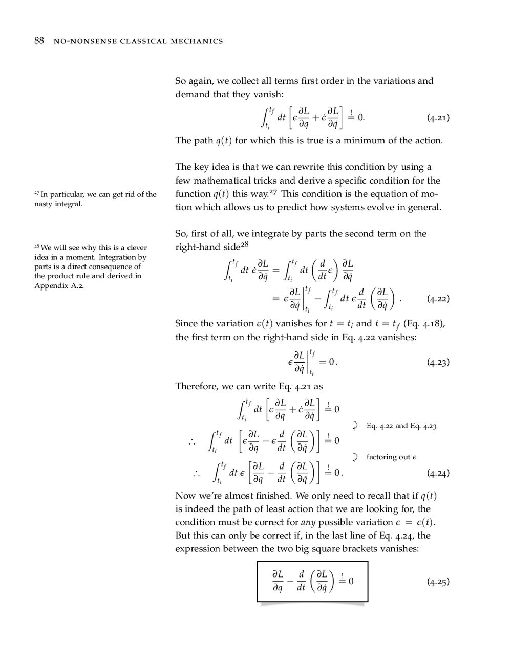
5. Cyclic coordinates and conservation laws in one glance
Suppose the Lagrangian does not depend on one of the coordinates $q_k$ (for instance, a central-force Lagrangian $L(r,\dot{r},\dot{\phi}) = \frac{1}{2}m(\dot{r}^2 + r^2\dot{\phi}^2) - V(r)$ does not contain the angle $\phi$ itself, only $\dot{\phi}$). Such a coordinate is called cyclic or ignorable. Then $\frac{\partial L}{\partial q_k} = 0$, so the Euler–Lagrange equation immediately reads:
$$\frac{d}{dt}\!\left(\frac{\partial L}{\partial \dot{q}_k}\right) = 0 \quad\Longrightarrow\quad p_k \equiv \frac{\partial L}{\partial \dot{q}_k} = \text{const.}$$For our central-force example, $p_\phi = \frac{\partial L}{\partial \dot{\phi}} = mr^2\dot{\phi} = \text{const}$—Kepler's equal-area law (conservation of angular momentum) falls out in a single line! Noether's theorem generalizes this observation to any continuous symmetry of the action, even when the symmetry mixes several coordinates.
Common questions
Why is the Lagrangian $L = T - V$ instead of $T + V$?
Because $T + V$ is total energy, whereas $L = T - V$ is the function whose stationary-action condition $\frac{d}{dt}(\partial L/\partial\dot{q}) = \partial L/\partial q$ produces $m\ddot{q} = -\partial V/\partial q$ with the right minus sign—and, at a deeper level, $\int(T-V)\,dt/\hbar$ is the quantum phase along each path in Feynman's path integral.
When does $L = T - V$ fail or need modification?
Velocity-dependent conservative forces still fit into a generalized Lagrangian—most famously a charge $q$ in an electromagnetic potential $(\phi, \mathbf{A})$ uses $L = \frac{1}{2}m\dot{\mathbf{x}}^2 - q\phi + q\dot{\mathbf{x}}\cdot\mathbf{A}$, whose Euler–Lagrange equation reproduces the Lorentz force $q(\mathbf{E} + \dot{\mathbf{x}}\times\mathbf{B})$ from Maxwell's electrodynamics! Relativistic free particles use $L = -mc^2\sqrt{1 - \dot{\mathbf{x}}^2/c^2}$ (which expands to $-mc^2 + \frac{1}{2}m\dot{\mathbf{x}}^2 + \dots$ at low speeds). Purely dissipative friction requires Rayleigh dissipation functions or coupling to microscopic bath degrees of freedom.
Are $q$ and $\dot{q}$ really independent variables?
As slots of the function $L(q,\dot{q},t)$, yes: at $t=0$ you are free to place a pendulum at any angle $\theta(0)$ and give it any push $\dot{\theta}(0)$ independently. Partial derivatives $\partial/\partial q$ and $\partial/\partial\dot{q}$ differentiate with respect to those slots first; only afterwards do you plug in a curve $q(t)$ and apply the total derivative $d/dt$.
Master the three formulations of mechanics
No-Nonsense Classical Mechanics builds Newtonian, Lagrangian, and Hamiltonian mechanics side by side—with 553 margin-annotated calculation steps, 1,124 sidenotes, solved comparisons on the harmonic oscillator and pendulum, Noether's theorem, and seven self-contained math appendices. See also our classical mechanics self-study plan and comparison with Taylor's Classical Mechanics.
Table of Contents (PDF) · Next step in this series: Annotated derivation of the Euler–Lagrange equation → · Noether's theorem →